Cogo Points from Text

Very often I come across survey drawings that have AutoCAD blocks and text representing the surveyed points.

If we want to create a surface in Civil 3D from these points we will need to add in the blocks (cross where the point was surveyed in image above) if they have levels. If they have no levels then second best is to add in the text (13.18) if this has a level. (the insertion point of the text wont be at the same location as the surveyed point but the difference this would make for a topo survey would be negligible in most cases). In my case neither has any level information - they are both at zero elevation. There is a workflow available that uses queries in Map 3D to raise the text up the elevation value in the text itself. I am going to show a different approach here using the AutoCAD Data Extraction command to create a csv file which contains the x ,y coordinates of the text and also the contents (elevation). we then import this back into C3D as cogo points.

First isolate all the 'elevation' pieces of text. Then type DATAEXTRACTION. On page 1 of 8 create a new extraction and save it. On 2 accept the defaults and click next. On 3 tick Text or MText - whichever the elevation text is, click next. On 4 on the RHS tick Geometry and Text, on the LH pane tick Contents, Position X & Position Y, click next.

On 5 untick Show Count Column and Show Name Column, click next. On 6 select 'Output to external data file' and choose a save location and file type. Step 7 is skipped if you just export to external file so on 8 just click finish. Job done. You now have a csv file with x,y,z for the survey points (with the point location at the insertion point of the text but close enough for a lot of surveys!)

You can then inport this back into Civil 3D as you would normally and create cogo points from it. One thing to be aware of is the first line of your csv file will be header info so delete this before trying to import into C3D or it will fail.

Not your Average Volume Calcs.

In some customised training recently I had a question on calculating the volume of material that was dumped on the side of an existing road. It turned out to be less straight forward than initially expected. The existing road is higher than the ground around it and original had a 2:1 embankment - that is all the information provided on the original condition. The fill material was dumped on top of this embankment. No survey existed for the original embankment so we had to somehow recreate the original ground level before we could calculate the volume of dumped material.

Belo is a screen shot of the current situation with a section through the fill to be quantified:

Manually drawn on one section below is the volume we need to calculate:

What we need to do is recreate the original field levels and road embankment at 1:1 to do our volume calculations - for simplicity we are going to assume the slope of the field continues in at the same grade towards the road:

 

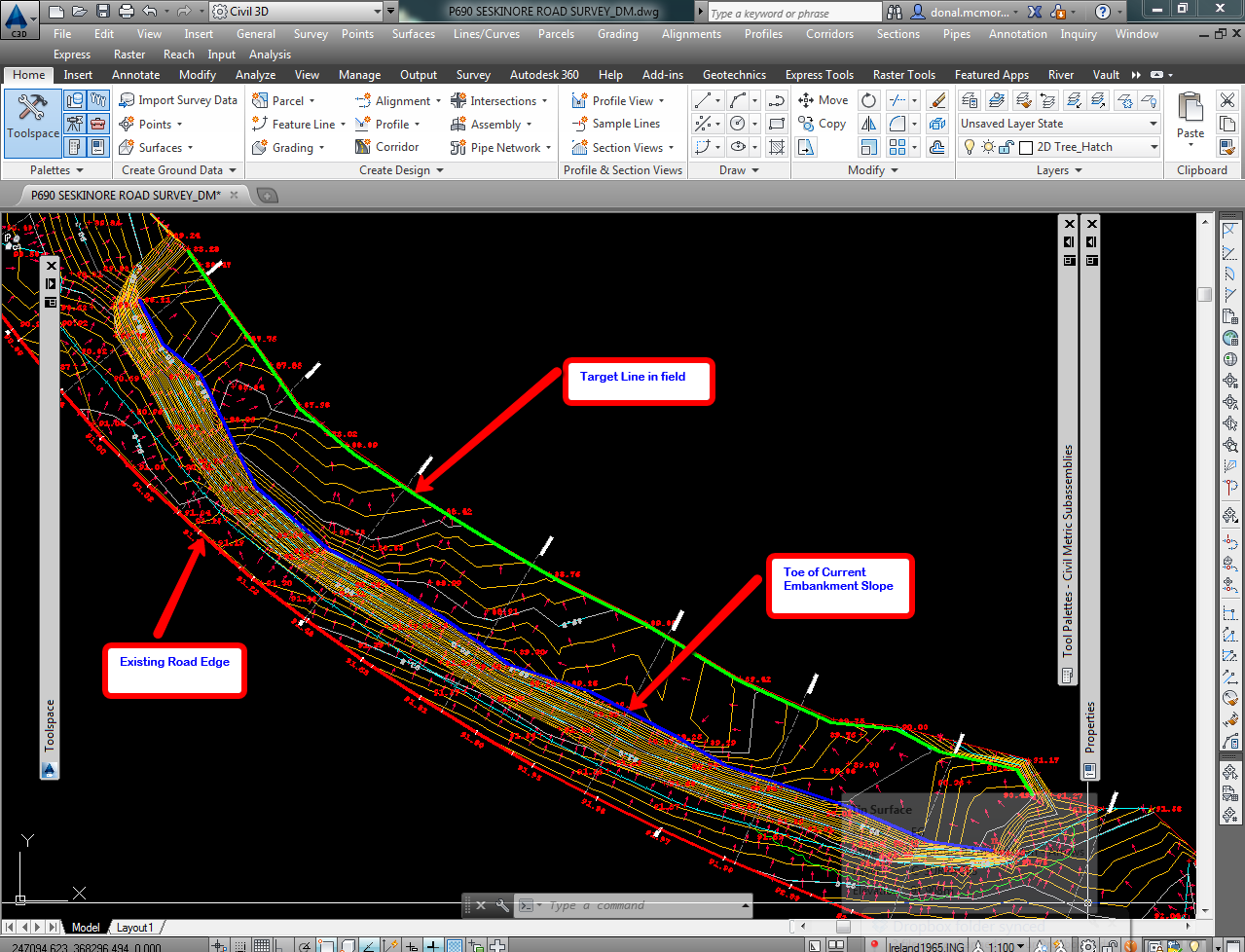
In plan below you can see the toe of current embankment - blue line. Red line is the road edge. 

To recreate the original field slope where the material was dumped we are going to use the overlaywidenmatchslope subassembly to build a corridor and get it to look at the existing field slope and continue this back in towards the road. Insertion point is toe of current slope and setting a target (green line) further out in the field will enable the assembly to calculate the slope of the field. 

The resulting corridor surface is shown below in purple. (actual slope may have been different but it is a good estimate). 

Next build another corridor with a linkslopetosurface subassembly. Alignment is existing road edge and existing profile. We will target the surface from the first corridor. 

The resulting corridor surface is shown below. We now have a good estimate of what the original ground levels were like before the material was dumped. 

Next to calculate the volumes we can define a material bounded by the three surfaces. 

 Volumes report below. 





Creating a 3D Ground Model from AutoCAD Data

If you have a topo survey in AutoCAD format only then the following video demonstrates a workflow for creating a ground model from that data in Civil 3D.

It is best to tidy up your drawing first and hide or remove any AutoCAD objects that you will not be using to define the ground model. This may include any objects with zero elevation (lines, text, blocks etc), or any other objects that you don't want to include. Performing this step first will make the Civil 3D part much easier...

Watch on highest quality for best results...

http://youtu.be/etGKbD_W86c

Sight Distance at Existing Junction

This post is an update to a previous one on the same topic, this one is hopefully more complete.


We have an existing junction and we need to improve the sight distance.

You can use a number of methods to check whether you are getting the required sight distance along your sightline.


1. You can create a profile along the sightline and check the sightline against the existing ground surface and see where the obstruction occurs:

or 2. use the visibility tool 'Point to Point' to check.

These methods only provide an answer along a single line. We can see in profile the depth of the earthworks that needs to be excavated. It would be useful to be able to show the extent of the obstructed view area in plan and get an idea of the extent of earthworks that would be required to provide visibility. To do this we can use a combination of dummy corridors and surfaces to give us the desired result.

First create a profile along your sightline in plan sampling the existing ground surface. Next create a profile from your eye (height 1.05m) to your target (height 0.26m) - see screen grab below.

Next create an assembly using the LinkOffsetandSlope on the Generic tab of the tool palettes.

Create the assembly wide enough to cover the area of interest:

Create a corridor from your sightline alignment, sightline profile and the above assembly. Create a surface from the corridor using top links.

Next create a volume surface using the Existing ground as the base surface and the corridor surface as the comparison. Set the surface style to 2D Solid Level Banding or similar.

In the surface properties for the volume surface set the analsyis to Elevations, create one range and set the max value for the range to zero.

The result will highlight in plan the area where the drivers view is obstructed by the existing ground surface.

Found this useful? Need to learn more? Check out our Advanced Junction Design course HERE

Surface Triangulation max angle problem

One new feature added to surfaces for 2013 is the ability to specify a maximum angle between surface triangle lines. This is supposed to build surfaces more intelligently by removing triangles that exceed the maximum angle and result in less erroneous triangulation.


See the following link for more info:


http://beingcivil.typepad.com/my_weblog/2012/04/autocad-civil-3d-2013-new-features-check-tin-for-max-angle.html


This is intended to be applied to triangles that make up the outer boundary of your surface only. However, after creating a surface (style - Border Only) from some LiDAR data last week I noticed there were 'holes' in the surface. See below:

After some searching I checked the max angle and set this to 'No' and rebuilt the surface and the holes disappeared.

So it would appear that the setting is applied to internal triangles also. (which it shouldn't be according to the help menu)

Stage Storage

I have to thank the guys from Autodesk who showed this a few weeks back at the Autodesk Industry Academy in Amsterdam....

I used to think that this tool was related to the Hydraflow Storm Sewers application and therefore not relevant to this part of the world due to differing hydrologic design methodologies.

However this is a stand alone tool that is a really simple and effective way of calculating the volume of a pond. You can calculate from either a surface or polylines.

Run the command and you are presented with the following dialog box:

In here you can click on Define to add data to use in the calculation - you can choose either surfaces or polylines. I have had a number of crashes when using surfaces but am unsure of whether this is an issue with the command or my surface. The alternative is to extract contours from your surface first and then use these polylines in the stage storage command instead. You can also export a .txt report of the analysis or insert a table of the results into the drawing using the buttons at the bottom of the dialog.

Wind Farm Access Roads - Hardstand Area Design

The following post forms part of an article written for this month's edition of AUGI World magazine on using Civil 3D for designing wind farm infrastructure, pg 54.

http://issuu.com/augi/docs/aw201205hr?mode=window&viewMode=doublePage


It follows on from a previous post on designing the access roads:
http://civilintentions.blogspot.com/2012/03/windfarm-access-roads-earthworks.html
Hardstand Area Design:

Hardstand areas are constructed to provide sufficient space for the cranes to operate during erection of the wind turbines. The hardstand areas must be large enough for the cranes to operate in and also provide storage space for materials.

The hardstand areas are effectively a widened region on the corridor. Typically the hardstand areas are flat and widen at right angles to the corridor, see image below. This can cause problems when targeting the hardstand widen alignments using an assembly on the centreline alignment. Civil 3D targets perpendicularly from the baseline alignment and will not model the hardstands correctly at the widen region.

There are a number of methods for modelling this type of widening.

a)  You could add offsets to your assembly and use the offset alignment to provide the offset value. This method gives mixed results when the widening is perpendicular to the main alignment.

b)  You could also create a featureline defining the edge of the hardstand and then use the grading tools to model the earthworks – this has the advantage of correctly modelling the grading in tight corners where the corridor would otherwise overlap. The disadvantage is that you have a number of ‘parts’ to your model and increased margin for error.

c)  The third method involves adding the hardstand alignments as new baselines to the corridor and applying earthworks assemblies along these baselines. This results in one object (the corridor) controlling the earthworks thus reducing the amount of ‘parts’ in your model. This is the method that has given the best results and the one we are going to look at here.

Step1: Create Hardstand Alignments and Profiles:

Create alignments defining the left and right edge of the hardstand and then create profiles along these alignments. As mentioned above, the hardstand areas need to be flat - the profiles along the edge of the hardstands need to be at the same level as the centreline profile. To achieve this we will use a dummy corridor to provide levels along the hardstand alignments.

To create the dummy corridor first create an assembly that has 0% grade and wide enough to extend beyond the extents of the hardstand. The LinkOffsetandSlope generic subassembly works well, see below.

Next build a dummy corridor along the centreline using the assembly. See below.

Create a surface from the corridor and finally a surface profile along each of the hardstand alignments sampling the dummy corridor surface. This gives our levels along the edge of the hardstands.

Step 2: Create Hardstand Assemblies:

The hardstand assemblies will be applied along the left and right hardstand alignments. The left and right assemblies will consist of the left and right earthworks subassemblies used in the main access road assembly.

Create your new assembly. Select the earthworks subassemblies from the main access road assembly. In the case below I am selecting the ditch, conditional cut/fill and generic subassemblies used to model the earthworks for the left side of the road.

Copy these to your hardstand assembly and repeat for the right hand side. Your finished assemblies will look something like the following:

Step 3: Add Baselines and Set Corridor Properties:

Next add the hardstand alignments to the main corridor as new base lines. In the corridor properties add a region to each of the new baselines for the chainages of the hardstand.

Anyone who has used corridors to model earthworks in tight corners will know that the downside is that the corridors do not resolve the overlap on the insides of bends similar to the grading tools– see screen grab below.

To resolve this issue we can use a workaround. In the corridor frequency for the hardstand regions set the sampling frequency to a value greater than the total length of the alignment and set the additional sampling frequencies to ’No’.

This will result in no automatic corridor sampling frequencies being applied to the region. We will then add in sampling stations manually at points along the region ensuring there is no corridor overlap in the earthworks.

This will not result in a perfectly modelled corridor but the differences in terms of volumes calculations are tiny in the grand scheme of things. The benefits achieved by having one corridor where you can easily make edits and create surfaces for volume calculations far outweighs those of having a 100% perfect model.

Wind Farm Design - Creating Geological Surfaces from Probed Depth Values

This post forms part of an article written for this month's edition of AUGI World magazine on how to use Civil 3D for designing wind farm infrastructure, pg 54.

http://issuu.com/augi/docs/aw201205hr?mode=window&viewMode=doublePage

Creating Geological Surfaces from Probed Depth Values:

Probed depths or borehole logs provide us with information on the subsurface geological layers for the site. When importing and using this data in Civil 3D there are a couple of issues that need to be looked at.

Issue 1: The surfaces created from the depth values in Civil 3D are of limited use. What we really need are the elevation values at each of the probe locations.  We need to convert the depth values into elevations.

Issue 2: Due to differing surface data resolutions (typically more points in the existing ground surface) the bottom of peat surface may not appear to accurately represent the geological layer – it may not ‘follow’ the lie of the land. See screen grab below. (You could in some cases see your subsurface extend above the existing ground in section). We need to create a surface that uses the probed depths and also ‘follows’ the existing ground in the areas in between where we do not have any probes.

There is workaround that has previously been posted on a number of blogs and forums that solves both of these issues. Here it is described as applied to a windfarm project - with a little bit of explanation of what is going on in the background from a Civil 3D point of view.

Solution:

1. Create a TIN surface from your probed peat depths – call it Probed Peat Depth.
2. Create a volume surface using the Existing Ground surface and the Probed Peat Depth surface – call it Peat Volume. The order in which you add the surfaces is important (base – Probed Peat Depths, Comparison – Existing Ground). You now have a volume surface that has depth values that are equal to the elevation for the bottom of peat.
3. Create a new TIN surface and call it Surface from Peat Volume. Paste in the Peat Volume surface. Pasting a volume surface into a TIN surface creates a surface with elevations equal to the depth values of the volume surface– we now have a TIN surface representing the bottom of peat.

The surface created in step 3 uses the probed peat depth values and follows the existing ground in between probes.  Note – this is not a true representation of the sub-surface geology but it is a good base to start with.

Surface Analysis Precision

This bugged me a while back and I meant to post about it.


I created a volume surface to show extent of cut/fill along my access road - red for cut and green for fill. I used the 2D Solid Level Banding surface style from the AutoCAD Civil 3D 2013 UKIE drawing template. I set my no. of ranges in the surface analysis to 2 which picks up the min and max levels on the surface and divides the level difference into two ranges.

All going well so far until I click ok and look at my surface... which appears to have 'holes' in it.

So why was this happening if I set it to automatically divide the surface into two ranges? The answer is in the surface style settings. The range precision is set to 1 which meant the max elevation for range 2 in my surface analysis stopped at 1m when in fact it was greater than that.

Setting the precision value to 0.001 and rerun the analysis solves the problem. Max elevation for range 2 now corrected to 1.293m.

The holes in my surface are no more...

The surface elevation analysis appears to begin at the absolute lowest elevation (ignoring precision) and work up to the max value (precision applied) - whereas I had always assumed that it found the absolute min and max levels first and then divided the difference into the specified number of ranges.

Reference Two Surfaces on one Label

I had a query recently about how to display both proposed and existing surface levels on one label/location and at set intervals along your alignment.


The answer involves creating a label style which consists of reference text. Reference text is a hidden gem and can be very useful in all sorts of situations. Basically it is a component added to a label which reads information from another Civil 3D object and displays that information in the label for the current object.


So in our case we will create an alignment label that is going to reference the level from two different surfaces. The other types of Civil 3D objects that you can reference are alignments, cogo points, parcels and profiles so you can end up getting quite creative with your labels...


To start, select your alignment, right click and select Edit Alignment Labels. Make a copy of one of the existing label styles.


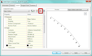
On the layout tab of the dialog box delete the existing components.

Now add a component as below and select Reference Text.

When asked for Type choose surface and give the component a name of 'EG Levels'.


Edit the text contents by clicking in the cell containing 'Label Text' and change this to reference Surface Elevation as shown below:

Repeat this adding another reference text component calling it FG Levels. In the text properties give this one a Y offset so the labels don't overlap.

Add the label to your alignment and set the increment as required. Now back in your drawing you should see something that looks like this:

The labels have been set up to reference a surface but we haven't told it which surface yet - this is why we see the question marks.


There is a bit of a trick to setting the referenced surfaces. If you click on a label it selects the whole set because that is what we have applied to the alignment - a label set. There is nowhere to set the reference objects in the label properties.


However, if you hold down control and click on a label it allows you to individually select a label and in the properties palette (right click and Properties) we can set the reference objects.

With a label selected click in the cell where it says <none> and move your cursor into the drawing, right click and select the surface from the list - do for both. Your label should now be referencing two surfaces.


To set the surfaces for the entire label set; select the label set, right click and isolate objects. Then hold down control and drag a selection box around all the labels, now in properties palette you can set the surfaces for all labels.


Just as an aside, the initial query I had was how to show proposed levels at the locations where the alignment crosses the existing contours. After much playing around I figured it wasn't possible without some programming but this was a suitable workaround.